Gaussian Processes for Classification and Regression: Introduction and Usage

Please note This post is mainly intended for my personal use. It is not peer-reviewed work and should not be taken as such.

TL;DR.

Like other Bayesian methods, Gaussian processes can be used for classification and regression in a way that also explicitly specifies the confidence interval of the predictions. You can also use Kernels to inform the algorithm with problem-specific data structure.

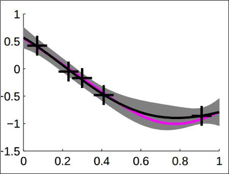Example of Gaussian Processes fitted on a couple of noisy observations (black crosses). Pink line shows actual function, black line shows the mean of the prediction, grey area indicates margin of error.
Source: Slides from UToronto (See refs)

Prereq: Probabilistic Intepretation of Linear Regression

The parameters that maximize:

• the log-likelihood that the curve fits the points, assuming that each point contains an error that follows the normal distribution and that this error is independent among samples.

Are the very same parameters that minimize:

• the least squares cost function, as used in ordinary least squares.

In other words least squares linear regression can be viewed as a maximum likelihood estimation (MLE) of the one set of parameters (theta, sigma) that maximize the likelihood that each sampled point in our dataset can be explained as a curve with parameters theta with some random noise (with mean on the curve itself and variance sigma).

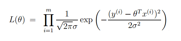Probabilistic Linear Regression: The likelihood of the parameters theta given targets y_i and samples x_i for a dataset containing m observations.
Adapted from: Stanford CS229 Lecture Notes

Prereq: Bayesian Regularization

A bayesian approach to a problem generally means treating every parameter configuration as a full distribution over values, and then using Bayes' rule to get the posterior probability of some configuration.

In other words, each parameter in the model is a bayesian random variable, with priors and the optimal value for the parameter is the value that maximizes its posterior distribution.

This allows for using external prior information to get a more accurate model, but more importantly, it acts as a regularizer because you are forced to take into account the priors of other parameter configurations too.

In other words, you multiply the value for the MLE/MAP estimation for a parameter configuration by the prior for that configuration.

Prereq: Kernels

Kernels are functions that return the inner product between two points in another vector space.

This is useful because many methods use inner products as a measure of similarity between two points and you can use kernels to discover the similarity of two points in another (higher-dimensional, nonlinear) space, without needing to directly calculate the projection of each point in that space.

Another explanation: A kernel is a function f(,) such that if you compute f(a,b) for every pair of elements in some S, you get a positive semidefinite matrix (i.e. a covariance matrix).

Properties of Multivariate Gaussians

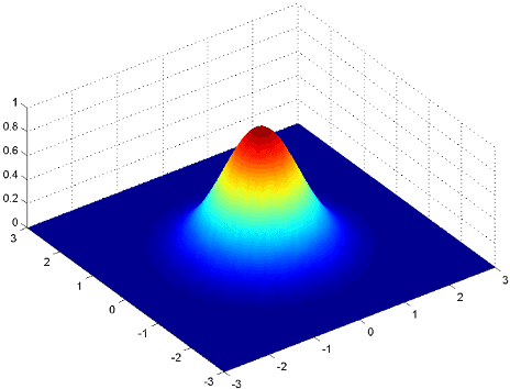2D Gaussian distribution with mean (0,0) and Identity Matrix for Covariances
Source: User Kghose at the English language Wikipedia (original link)

Given a N-dimensional random variable X that follows a (multivariate) Gaussian distribution:

• The density function sums to one. (Obvious but it's worth remembering)

• Any linear combination of its components is also Gaussian.

• The marginal densities of any subset of elements are also Gaussians.

• The conditional densities of any subset of elements given another subset is also Gaussian.

• The sum of independent Gaussian random variables is also Gaussian.

• If the individual components of X are each normally distributed and they are independent, then X is a multivariate Gaussian.

Probability distributions over functions with finite domains

If you have a finite number of inputs (say the number of samples, m), you can view the mapping of features to target values as a function, but you can represent it using a m-dimensional vector of real numbers, one for each input.

But since this is just an n-dimensional array, you can view it as a distribution over values, rather than as just a single, static, set of values.

This is what is meant by a distribution over functions with finite domains.

Gaussian Processes

A Gaussian Process is the generalization of the above (distribution over functions with finite domains) in the infinite domain.

This is achieved by sampling mean functions m(x_1) and covariance functions k(x_1,x_2) that return the mean to be used to generate the Gaussian distribution to sample the first element and also the covariance function between every pair of variables.

The interesting thing is that, while any function is a valid mean function, not every function is a valid covariance.

Only a certain type of function can be used as a covariance function for a multivariate Gaussian distribution: a Kernel.

Usage in Classification/Regression

As in the probabilistic linear regression case, we will assume our samples in the training set can be modelled by some function Z plus some gaussian noise.

So when doing regression, we actually are trying to find out the most likely distribution (i.e. highest posterior probability) of the values in the test set given the values in the training set.

But if we take function Z itself to be a Gaussian Process, we can use all those properties of multivariate gaussians stated earlier (sum of gaussians is also gaussian, conditional distribution of a subset is also gaussian).

Such a choice of assumptions allows us to calculate the posterior distribution (or just the most likely values) for the test targets, given the training targets.

Gaussian Processes for Regression are a generalization of Bayesian Linear regression.

For classification problems, one simple way to adapt gaussian processes is to choose a 0-1 loss (i.e. punish false positives and false negatives equally), normalize the target into a 0-1 interval (e.g. using the logistic function) so that it can be viewed as a probability and choosing some threshold value for actual classification.

Sparse Gaussian Processes

Gaussian processes are powerful general-purpose models but fitting the model to training data is potentially very time-consuming (exponential time on the number of samples) due to operations such as inverting the covariance matrix.

Sparse gaussian processes refer to techniques in which only a subset of the training samples deemed more informative is selected for training. This presents a tradeoff between training time and model accuracy.

References

• Stanford CS229: Gaussian Processes

• Quora: What are the advantages of Bayesian methods over frequentist methods in web data?

  • See the first answer for a good answer on how Bayesian priors can be used as regularizers.

• Stanford CS229: The Multivariate Gaussian Distribution

• UToronto: Introduction to Gaussian Processes, Slides by Iain Murray

• Mathematical Monk: Gaussian coordinates do not imply multivariate Gaussian

  • This is just one of the videos on this theme. This guy has 11 videos dealing with Gaussian Processes overall.