Introduction to AUC and Calibrated Models with Examples using Scikit-Learn
Last updated:
- Scores vs Probabilities
- Calibration vs Discrimination
- Calibration makes decision-making easier
- Sigmoid vs Isotonic calibration
- Example: Calibrate discrete classifier with CalibratedClassifierCV
- Example: Calibrate a continous classifier
- Natively Calibrated classifiers
- Do not use AUC if
This was inspired by an earlier (2017) podcast episode by Linear Digressions.
Scores vs Probabilities
The score you get from a binary classifier (that outputs a number between 0 and 1) is not necessarily a well-calibrated probability.
This is not always a problem because it generally sufices to have scores that correctly order the samples, even if they don't actually correspond to probabilities.
Example: A logistic regression binary classifier naturally produces scores that are actual probabilities (i.e. if it reports a score of 0.9 for an instance, it means that that instance would be 1 90% of the time and 0 10% of the time.)
Calibration vs Discrimination
| Discrimination | Calibration |
|---|---|
| Measures how often a classifier ranks true 1s higher than true 0s | Measures how much classifier scores align with actual (empirical) probabilities |
Discrimination: For every two samples A and B, where the true value of A is 1 and B is 0, how often does your model gives a higher score to A than to B? It can be measured by the AUC.
Calibration: How well model output actually matches the probability of the event. It can be measured by the Hosmer-Lemeshow statistic and by the Brier Score.
If order to understand how they differ, imagine the following:
You have a model that gives a AUC score of 0.52 to every
Trueinstance and 0.51 to everyFalse. It will have perfect discrimination (AUC = 1.0) but very poor calibration (i.e. the score has very little correlation with actual event probability).
Calibration makes decision-making easier
Calibration is important in problems where someone needs to make decisions based on model outputs
In many cases, the output scores of these models are used to drive actions and help people make decisions.
The natural way to do this is to use thresholds, i.e. define a cutoff value for the scores, and act on the instances that cross that threshold.
Examples:
If your model outputs credit default probabilities, it may the company's policy to contact every customer whose default risk is over 0.6.
If your model outputs risk of heart failure in the next 3 months, the doctors (or medical guidelines) may need to act on the people whose risk is above 0.5, to prevent the event from taking place.
If your model's calibration isn't up to scratch, you'll mislead anyone taking action based on its outputs.
Also, calibrated predictions help users and stakeholders build trust in your model.
Because the results correlate directly with the actual confidence those predictions carry.
In other words, a score of 0.8 given by a calibrated classifier actually means that that instance has an 80% chance of being True.
Sigmoid vs Isotonic calibration
Sigmoid calibration is also called Platt's Scaling
Sigmoid Calibration simply means to fit a Logistic Regression classifier using the (0 or 1) outputs from your original model.
Isotonic Calibration (also called Isotonic Regression) fits a piecewise function to the outputs of your original model instead.
Example: Calibrate discrete classifier with CalibratedClassifierCV
Here, we are just using CalibratedClassifierCV to turn a discrete binary classifier into one that outputs well-calibrated continous probabilities.
import numpy as np

from sklearn.datasets import make_classification
from sklearn.svm import LinearSVC
from sklearn.metrics import brier_score_loss
from sklearn.model_selection import train_test_split
from sklearn.calibration import CalibratedClassifierCV,calibration_curve
from sklearn import metrics

import matplotlib.pyplot as plt

np.random.seed(42)

# class_sep set to 0.5 to make it a little more difficult
X, y = make_classification(n_samples=9000,n_features=20,class_sep=0.5)

X_train, X_test, y_train, y_test = train_test_split(X, y, test_size=0.20)

clf = CalibratedClassifierCV(LinearSVC(),method='isotonic',cv=2)
clf.fit(X_train,y_train)

y_preds = clf.predict_proba(X_test)
preds = y_preds[:,1]

# also predict discrete labels for comparison
discrete_preds = clf.predict(X_test)

## PLOT CURVE

plt.clf()

ax = plt.gca()

clf_score = brier_score_loss(y_test, preds, pos_label=1)

fraction_of_positives, mean_predicted_value = calibration_curve(y_test, preds, n_bins=20)
ax.plot(mean_predicted_value, fraction_of_positives, "s-", label="Sigmoid Calibration (Brier loss={:.2f})".format(clf_score))

clf_score = brier_score_loss(y_test, discrete_preds, pos_label=1)

fraction_of_positives, mean_predicted_value = calibration_curve(y_test, discrete_preds, n_bins=20)
ax.plot(mean_predicted_value, fraction_of_positives, "s-", label="Discrete predictions (Brier loss={:.2f})".format(clf_score))
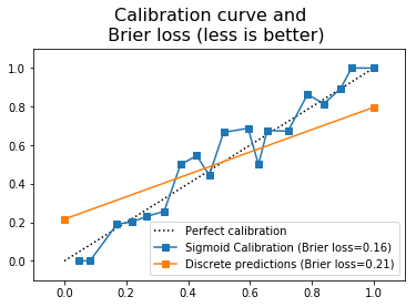 Calibration turned the discrete classifier into a continuous classifier
 whose outputs can be roughly interpreted as probabilities
Example: Calibrate a continous classifier
In this example, let's see how to calibrate a model that outputs continuous (real-valued) numbers, so that they become calibrated probabilities.
In this example, we see how GradientBoostingClassifier outputs predictions that are not very well calibrated, (even though it has a predict_proba() method):
import numpy as np

from sklearn.datasets import make_classification
from sklearn.metrics import brier_score_loss,log_loss
from sklearn.model_selection import train_test_split
from sklearn.calibration import CalibratedClassifierCV,calibration_curve
from sklearn import metrics
from sklearn.ensemble import GradientBoostingClassifier

import matplotlib.pyplot as plt

np.random.seed(42)

X, y = make_classification(n_samples=150000,n_features=10,n_informative=5,n_redundant=5, class_sep=0.05)

X_train, X_test, y_train, y_test = train_test_split(X, y, test_size=0.60)

clf = GradientBoostingClassifier()
clf.fit(X_train,y_train)

# prefit means that the underlying classifier has already been fitted
ccv_sig = CalibratedClassifierCV(clf,cv='prefit',method='sigmoid')
ccv_sig.fit(X_train,y_train)

ccv_iso = CalibratedClassifierCV(clf,cv='prefit',method='isotonic')
ccv_iso.fit(X_train,y_train)

# ṔLOT THE RELIABILITY CURVES FOR BOTH CALIBRATION TYPES

plt.clf()

fig, axes = plt.subplots(1,2,sharey=True)

# SIGMOID CALIBRATION

ccv_preds_sig = ccv_sig.predict_proba(X_test)[:,1]

ax=axes[0]

clf_score = brier_score_loss(y_test, clf_preds, pos_label=1)

fraction_of_positives, mean_predicted_value = calibration_curve(y_test, clf_preds, n_bins=30)
ax.plot(mean_predicted_value, fraction_of_positives, "r-", label="No Calibration (Brier loss={:.3f})".format(clf_score))

clf_score = brier_score_loss(y_test, ccv_preds_sig, pos_label=1)

fraction_of_positives, mean_predicted_value = calibration_curve(y_test, ccv_preds_sig, n_bins=30)
ax.plot(mean_predicted_value, fraction_of_positives, "b-", label="Sigmoid Calibration (Brier loss={:.3f})".format(clf_score))

# ISOTONIC CALIBRATION

ccv_preds_iso = ccv_iso.predict_proba(X_test)[:,1]

ax=axes[1]

clf_score = brier_score_loss(y_test, clf_preds, pos_label=1)

fraction_of_positives, mean_predicted_value = calibration_curve(y_test, clf_preds, n_bins=30)
ax.plot(mean_predicted_value, fraction_of_positives, "r-", label="No Calibration (Brier loss={:.3f})".format(clf_score))

clf_score = brier_score_loss(y_test, ccv_preds_iso, pos_label=1)

fraction_of_positives, mean_predicted_value = calibration_curve(y_test, ccv_preds_iso, n_bins=30)
ax.plot(mean_predicted_value, fraction_of_positives, "b-", label="Isotonic Calibration (Brier loss={:.3f})".format(clf_score))
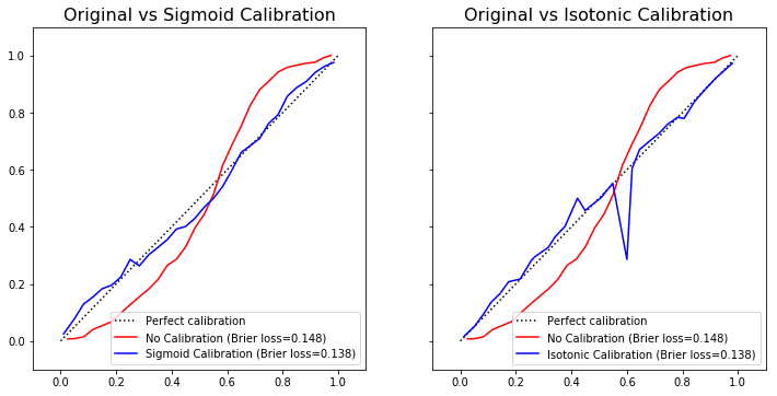 GradientBoostingClassifier already supports
 predict_proba but that doesn't mean that its outputs are well calibrated.
Different calibration techniques may yield different outcomes.
Natively Calibrated classifiers
Some classifiers output calibrated probabilities out of the box, including:
XGBoostClassifier, but only when using the following objective functions (see all available objective functions here)
'binary:logistic'for bianry classification'multi:softprob'for multiclass classification
Do not use AUC if
You want scores you can interpret at probabilities
AUC may be higher for models that don't output calibrated probabilities.
In other words, if you want to measure risk of something happening (heart disease, credit default, etc), AUC is not the metric for you.
You are still selecting features
If you want to select features by looking at AUC of models trained with them, you may be misled by AUC.
This is because a feature's importance may not overly change the discrimination of the model even though it may increase the accuracy in the probabilities output.
You want to create stratified groups depending on output scores
If your model outputs credit default risk scores, one thing you may be asked to do is to group those clients into ratings. For example, you would want to assign credit rating "A" to clients on bottom 10% of default risk, "B" to clients having 10%-20% risk, and so on, until "H".
In other words, if you need to get the order of your scores right, AUC isn't a good metric to help you with that (because it measures discrimination, not calibration).
References
Cook 2007: Use and misuse of the ROC Curve in Risk Prediction
- AUC is called the c-Statistic in the medical literature.