Visualizing Machine Learning Models: Examples with Scikit-learn, XGB and Matplotlib
Last updated:- Plot ROC Curve and AUC
- Plot Grid Search Results
- Plot XGBoost Feature Importance
- Plot categorical feature importances
- Plot confusion matrix
Plot ROC Curve and AUC
For more detailed information on the ROC curve see AUC and Calibrated models
The ROC curve and the AUC (the Area Under the Curve) are simple ways to view the results of a classifier.
The ROC curve is good for viewing how your model behaves on different levels of false-positive rates and the AUC is useful when you need to report a single number to indicate how good your model is.
import matplotlib.pyplot as plt
from sklearn import metrics
from sklearn.linear_model import LogisticRegression

# load data
X_train, X_test, y_train, y_test = load_my_data()

# model can be any trained classifier that supports predict_proba()
clf = LogisticRegression()
clf.fit(X_train, y_train)

y_preds = clf.predict_proba(X_test)

# take the second column because the classifier outputs scores for
# the 0 class as well
preds = y_preds[:,1]

# fpr means false-positive-rate
# tpr means true-positive-rate
fpr, tpr, _ = metrics.roc_curve(y_test, preds)

auc_score = metrics.auc(fpr, tpr)

# clear current figure
plt.clf()

plt.title('ROC Curve')
plt.plot(fpr, tpr, label='AUC = {:.2f}'.format(auc_score))

# it's helpful to add a diagonal to indicate where chance
# scores lie (i.e. just flipping a coin)
plt.plot([0,1],[0,1],'r--')

plt.xlim([-0.1,1.1])
plt.ylim([-0.1,1.1])
plt.ylabel('True Positive Rate')
plt.xlabel('False Positive Rate')

plt.legend(loc='lower right')
plt.show()
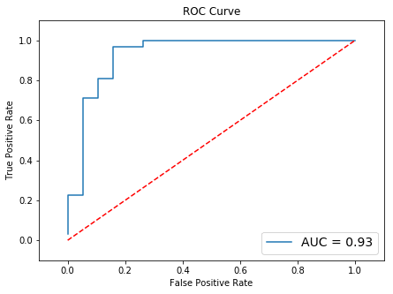 Results may vary, especially in real-life problems.
 This is a dummy dataset.
Plot Grid Search Results
It is useful to view the results for all runs of a grid search.
See the full output on this jupyter notebook
Here is one way to do it: create multiple plots using plt.subplots() and plot the results for each with the title being the current grid configuration.
import matplotlib.pyplot as plt
import math

from sklearn import metrics

from sklearn.model_selection import ParameterGrid, train_test_split
from sklearn.pipeline import Pipeline
from sklearn.decomposition import PCA
from sklearn.ensemble import GradientBoostingClassifier
from sklearn.datasets import make_classification

# load data
X, y = make_classification(n_samples=10000,
                           n_features=25,
                           n_redundant=10,
                           n_repeated=5,
                           class_sep=0.2,
                           flip_y=0.1)

X_train, X_test, y_train, y_test = train_test_split(X, y, test_size=0.35)

# out pipeline has uses PCA for preprocessing then
# a gradient boosting classifier
param_grid = [
    {
        'pca__n_components':[5,10,20],
        'clf__n_estimators':[5,20,50,100,200],
        'clf__max_depth':[1,2,3,4]
    }
]

pipeline = Pipeline([
    ('pca',PCA()),
    ('clf',GradientBoostingClassifier())
])
Once the pipeline and the parameter grid are built (previous code block), proceed as follows:
Create a plot to hold all subplots
Loop over each run of the grid using
ParameterGridIn each loop, do:
- Train/score the classifier for the current parameter configuration.
- Plot the performance for the current configuration.
# now plotting:

num_cols = 3
num_rows = math.ceil(len(ParameterGrid(param_grid)) / num_cols)

# create a single figure
plt.clf()
fig,axes = plt.subplots(num_rows,num_cols,sharey=True)
fig.set_size_inches(num_cols*5,num_rows*5)

for i,g in enumerate(ParameterGrid(param_grid)):

    pipeline.set_params(**g)
    pipeline.fit(X_train,y_train)

    y_preds = pipeline.predict_proba(X_test)

    # take the second column because the classifier outputs scores for
    # the 0 class as well
    preds = y_preds[:,1]

    # fpr means false-positive-rate
    # tpr means true-positive-rate
    fpr, tpr, _ = metrics.roc_curve(y_test, preds)

    auc_score = metrics.auc(fpr, tpr)

    ax = axes[i // num_cols, i % num_cols]

    # don't print the whole name or it won't fit
    ax.set_title(str([r"{}:{}".format(k.split('__')[1:],v) for k,v in g.items()]),fontsize=9)
    ax.plot(fpr, tpr, label='AUC = {:.3f}'.format(auc_score))
    ax.legend(loc='lower right')

    # it's helpful to add a diagonal to indicate where chance
    # scores lie (i.e. just flipping a coin)
    ax.plot([0,1],[0,1],'r--')

    ax.set_xlim([-0.1,1.1])
    ax.set_ylim([-0.1,1.1])
    ax.set_ylabel('True Positive Rate')
    ax.set_xlabel('False Positive Rate')

plt.gcf().tight_layout()
plt.show()
The result will look like this:
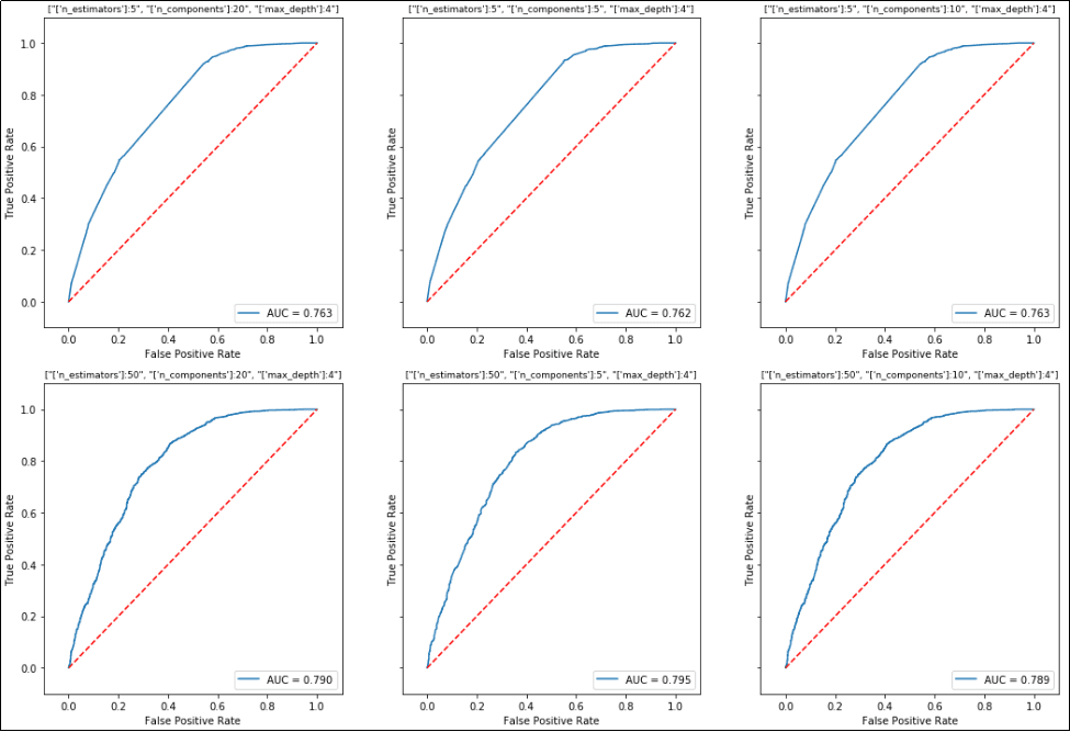 One plot is drawn for each configuration in the grid search.
 Note that the title for each plot is the configuration of the grid at that step.
Plot XGBoost Feature Importance
Using data from the Kaggle titanic competition
Use zip(data.columns,clf.feature_importances_) to make a dictionary linking variable names (in a pandas dataframe) and the variable importances:
Full code can be found here: plot-importances-xgb.ipynb
import matplotlib.pyplot as plt
import numpy as np
import pandas as pd

from sklearn.model_selection import train_test_split

from xgboost import XGBClassifier

# this is the titanic train set
df = pd.read_csv('train.csv')

# let's just use 'Fare' and 'Age' features
data=df[['Age','Fare']]
target = df['Survived']

X_train, X_test, y_train, y_test = train_test_split(data.values, target.values, test_size=0.4)

clf = XGBClassifier()
clf.fit(X_train,y_train)

# build importance data
importance_data = sorted(list(zip(data.columns,clf.feature_importances_)),key=lambda tpl:tpl[1],reverse=True)

xs = range(len(importance_data))
labels = [x for (x,_) in importance_data]
ys = [y for (_,y) in importance_data]

# plot
plt.clf()
plt.bar(xs,ys,width=0.5)
plt.xticks(xs,labels)
plt.show()
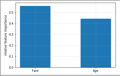 Feature importance plot for a model that uses just two featues
Plot categorical feature importances
Using data from the Kaggle titanic competition
As above, we build variable importances but we also merge together one-hot-encoded variables in the dataframe.
XGBoost treats one-hot-encoded variables separately, but it's likely that you want to see the full importance for each categorical variable as a whole.
import matplotlib.pyplot as plt
import numpy as np
import pandas as pd

from sklearn.model_selection import train_test_split

from xgboost import XGBClassifier

# this is the titanic train set
df = pd.read_csv('train.csv')

# select the columns we will use
df = df[['Pclass','Sex','SibSp','Embarked','Age','Fare','Survived']]

# one-hot-encode categorical variables
# note that we use each variable name as the prefix for dummy variables
df = pd.concat([df,pd.get_dummies(df['Pclass'], prefix='Pclass',dummy_na=True)],axis=1).drop(['Pclass'],axis=1)
df = pd.concat([df,pd.get_dummies(df['Sex'], prefix='Sex',dummy_na=True)],axis=1).drop(['Sex'],axis=1)
df = pd.concat([df,pd.get_dummies(df['SibSp'], prefix='SibSp',dummy_na=True)],axis=1).drop(['SibSp'],axis=1)
df = pd.concat([df,pd.get_dummies(df['Embarked'], prefix='Embarked',dummy_na=True)],axis=1).drop(['Embarked'],axis=1)

data=df.drop(['Survived'],axis=1)
target = df['Survived']

X_train, X_test, y_train, y_test = train_test_split(data.values, target.values, test_size=0.4)

clf = XGBClassifier()
clf.fit(X_train,y_train)
at this point, we will modify the feature importances dict so that we get the sum of the importances for each categorical variable:
# clf should be a trained classifier
# data is a dataframe with ONLY features, no target variables od IDs

# define the base names for each variables
categorical_columns_names = ['Pclass','Sex','SibSp','Embarked']

importances_dict = dict(zip(data.columns,clf.feature_importances_))

for column_name in categorical_columns_names:

    all_values_sum = 0

    for key,value in list(importances_dict.items()):
        if key.startswith(column_name):
            all_values_sum += importances_dict[key]
            del(importances_dict[key])

    importances_dict[column_name] = all_values_sum


# now we proceed the same as in the previous example, but using the
# modified importance we calculated above
importance_data = sorted(list(importances_dict.items()),key=lambda tpl:tpl[1],reverse=True)

xs = range(len(importance_data))
labels = [x for (x,_) in importance_data]
ys = [y for (_,y) in importance_data]

# plot
plt.bar(xs,ys,width=0.5)
plt.xticks(xs,labels)
plt.show()
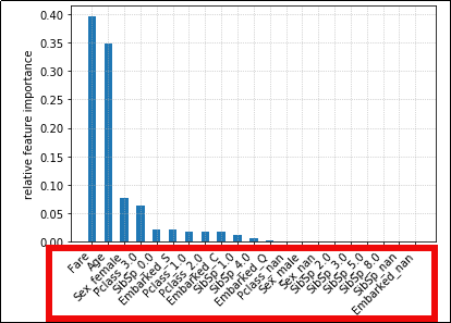 When we one-hot-encode categorical
 and use them in Gradient Boosting,
importance is calculated individually
for each possible category value. This
makes it hard to see importances for each
categorical variable.
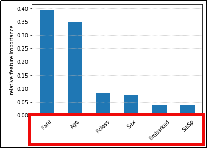 We can alter the importance
 values so that the sum for all values
in a category is shown.
(Much easier to visualize)
Plot confusion matrix
A more complete way to plot confusion matrices is available in library python-ds-util
Confusion matrices are useful to inform what kinds of errors your models tend to make.
They work for binary classification and for multi-class classification too.
Example: Train an xgboost classifier on dummy multi-class data and plot confusion matrix, with labels and a colorbar to the right of the plot:
- Part 1: Train and score the model using dummy data
import numpy as np
import itertools

import matplotlib.pyplot as plt

from sklearn.datasets import make_classification
from sklearn.model_selection import train_test_split
from sklearn.metrics import confusion_matrix

from xgboost import XGBClassifier

# using random data for this exaple
X, y = make_classification(
    n_samples=10000,
    n_features=25,
    n_informative=10,
    n_redundant=0,
    n_classes=5)

class_names = ['class-1','class-2','class-3','class-4','class-5']

X_train, X_test, y_train, y_test = train_test_split(X, y, test_size=0.33)

clf = XGBClassifier()
clf.fit(X_train,y_train)

y_pred = clf.predict(X_test)
- Part 2: Build confusion matrix data and plot image
matrix = confusion_matrix(y_test,y_pred)

plt.clf()

# place labels at the top
plt.gca().xaxis.tick_top()
plt.gca().xaxis.set_label_position('top')

# plot the matrix per se
plt.imshow(matrix, interpolation='nearest', cmap=plt.cm.Blues)

# plot colorbar to the right
plt.colorbar()

fmt = 'd'

# write the number of predictions in each bucket
thresh = matrix.max() / 2.
for i, j in itertools.product(range(matrix.shape[0]), range(matrix.shape[1])):

    # if background is dark, use a white number, and vice-versa
    plt.text(j, i, format(matrix[i, j], fmt),
         horizontalalignment="center",
         color="white" if matrix[i, j] > thresh else "black")

tick_marks = np.arange(len(class_names))
plt.xticks(tick_marks, class_names, rotation=45)
plt.yticks(tick_marks, class_names)
plt.tight_layout()
plt.ylabel('True label',size=14)
plt.xlabel('Predicted label',size=14)
plt.show()
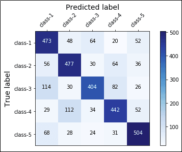 A complete confusion matrix for a 5-class
 classification problem.
The main diagonal represents accurate
predictions while other squares represent
misclassifications.
Full code available on this link