Evaluation Metrics for Ranking problems: Introduction and Examples
Last updated:
- Ranking Problems
- Sample dataset (Ground Truth)
- Precision @k
- Recall @k
- F1 @k
- AP: Average Precision
- DCG: Discounted Cumulative Gain
- NDCG: Normalized Discounted Cumulative Gain
- MAP: Mean Average Precision
- Average Precision @k
- DCG vs NDCG
Ranking Problems
In many domains, data scientists are asked to not just predict what class/classes an example belongs to, but to rank classes according to how likely they are for a particular example.
| Classification | Ranking |
|---|---|
| Order of predictions doesn't matter | Order of predictions does matter |
In the real world, resources are limited and people using model predictions have limited time. So they usually need to prioritize, rank results.
Some domains where this is particularly noticeable:
Search engines: Predict which documents match a query on a search engine.
Tag suggestion for Tweets: Predict which tags should be assigned to a tweet.
Image label prediction: Predict what labels should be suggested for a picture.
If your machine learning model produces a real-value for each of the possible classes, you can turn a classification problem into a ranking problem.
In other words, if you predict scores for a set of examples and you have a ground truth, you can order your predictions from highest to lowest and compare them with the ground truth:
Search engines: Do relevant documents appear up on the list or down at the bottom?
Tag suggestion for Tweets: Are the correct tags predicted with higher score or not?
Image label prediction: Does your system correctly give more weight to correct labels?
In the following sections, we will go over many ways to evaluate ranked predictions with respect to actual values, or ground truth.
Sample dataset (Ground Truth)
We will use the following dummy dataset to illustrate examples in this post:
| ID | Actual Relevance |
Text |
|---|---|---|
| 00 | Relevant (1.0) | Lorem ipsum dolor sit amet, consectetur adipiscing elit. |
| 01 | Not Relevant (0.0) | Nulla non semper lorem, id tincidunt nunc. |
| 02 | Relevant (1.0) | Sed scelerisque volutpat eros nec tincidunt. |
| 03 | Not Relevant (0.0) | Fusce vel varius erat, vitae elementum lacus. |
| 04 | Not Relevant (0.0) | Donec vitae lobortis odio. |
| 05 | Relevant (1.0) | Quisque congue suscipit augue, congue porta est pretium vel. |
| 06 | Relevant (1.0) | Donec eget enim vel nisl feugiat tincidunt. |
| 07 | Not Relevant (0.0) | Nunc vitae bibendum tortor. |
Documents 0,2,5 and 6 are relevant; 1,3,4 and 7 are not
Precision @k
Precision means: "of all examples I predicted to be TRUE, how many were actually TRUE?"
\(Precision\) \(@k\) ("Precision at \(k\)") is simply Precision evaluated only up to the \(k\)-th prediction, i.e.:
$$ \text{Precision}@k = \frac{true \ positives \ @ k}{(true \ positives \ @ k) + (false \ positives \ @ k)} $$
scores (Sorted)
| k | Document ID |
Predicted Relevance |
Actual Relevance |
Precision @k |
|---|---|---|---|---|
| 1 | 06 | 0.90 | Relevant (1.0) | 1.0 |
| 2 | 03 | 0.85 | Not Relevant (0.0) | 0.50 |
| 3 | 05 | 0.71 | Relevant (1.0) | 0.66 |
| 4 | 00 | 0.63 | Relevant (1.0) | 0.75 |
| 5 | 04 | 0.47 | Not Relevant (0.0) | 0.60 |
| 6 | 02 | 0.36 | Relevant (1.0) | 0.66 |
| 7 | 01 | 0.24 | Not Relevant (0.0) | 0.57 |
| 8 | 07 | 0.16 | Not Relevant (0.0) | 0.50 |
from highest to lowest
Example: Precision @1
I.e. what Precision do I get if I only use the top 1 prediction?
$$ \text{Precision}@1 = \frac{\text{true positives} \ @ 1}{(\text{true positives} \ @ 1) + (\text{false positives} \ @ 1)} $$
$$ \hphantom{\text{Precision}@1} = \frac{\text{true positives considering} \ k=1}{(\text{true positives considering} \ k=1) + \\ (\text{false positives considering} \ k=1)} $$
$$ = \frac{1}{1 + 0} $$
$$ =1 $$
Example: Precision @4
Similarly, \(Precision@4\) only takes into account predictions up to \(k=4\):
$$ \text{Precision}@4 = \frac{\text{true positives} \ @ 4}{\text{(true positives} \ @ 4) + (\text{false positives} \ @ 4)} $$
$$ \hphantom{\text{Precision}@4} = \frac{\text{true positives considering} \ k=4}{(\text{true positives considering} \ k=4) + \\ (\text{false positives considering} \ k=4)} $$
$$ = \frac{3}{3 + 1} $$
$$ =0.75 $$
Example: Precision @8
Finally, \(Precision@8\) is just the precision, since 8 is the total number of predictions:
$$ \text{Precision}@8 = \frac{\text{true positives} \ @ 8}{(\text{true positives} \ @ 8) + (\text{false positives} \ @ 8)} $$
$$ \hphantom{\text{Precision}@8} = \frac{\text{true positives considering} \ k=8}{(\text{true positives considering} \ k=8) + \\ (\text{false positives considering} \ k=8)} $$
$$ = \frac{4}{4 + 4} $$
$$ =0.5 $$
Recall @k
Recall means: "of all examples that were actually TRUE, how many I predicted to be TRUE?"
\(Recall\) \(@k\) ("Recall at \(k\)") is simply Recall evaluated only up to the \(k\)-th prediction, i.e.:
$$ \text{Recall}@k = \frac{true \ positives \ @ k}{(true \ positives \ @ k) + (false \ negatives \ @ k)} $$
scores (Sorted)
| k | Document ID | Predicted Relevance |
Actual Relevance |
Recall @k |
|---|---|---|---|---|
| 1 | 06 | 0.90 | Relevant (1.0) | 0.25 |
| 2 | 03 | 0.85 | Not Relevant (0.0) | 0.25 |
| 3 | 05 | 0.71 | Relevant (1.0) | 0.50 |
| 4 | 00 | 0.63 | Relevant (1.0) | 0.75 |
| 5 | 04 | 0.47 | Not Relevant (0.0) | 0.75 |
| 6 | 02 | 0.36 | Relevant (1.0) | 1.0 |
| 7 | 01 | 0.24 | Not Relevant (0.0) | 1.0 |
| 8 | 07 | 0.16 | Not Relevant (0.0) | 1.0 |
ordered from highest to lowest
Example: Recall @1
I.e. what Recall do I get if I only use the top 1 prediction?
$$ \text{Recall}@1 = \frac{\text{true positives} \ @ 1}{(\text{true positives} \ @ 1) + (\text{false negatives} \ @ 1)} $$
$$ \hphantom{\text{Recall}@1} = \frac{\text{true positives considering} \ k=1}{(\text{true positives considering} \ k=1) + \\ (\text{false negatives considering} \ k=1)} $$
$$ = \frac{1}{1 + 3} $$
$$ =0.25 $$
Example: Recall @4
Similarly, \(Recall@4\) only takes into account predictions up to \(k=4\):
$$ \text{Recall}@4 = \frac{true \ positives \ @ 4}{(true \ positives \ @ 4) + (false \ negatives \ @ 4)} $$
$$ \hphantom{\text{Recall}@4} = \frac{\text{true positives considering} \ k=4}{(\text{true positives considering} \ k=4) + \\ (\text{false negatives considering} \ k=4)} $$
$$ = \frac{3}{3 + 1} $$
$$ =0.75 $$
Example: Recall @8
$$ \text{Recall}@8 = \frac{true \ positives \ @ 8}{(true \ positives \ @ 8) + (false \ negatives \ @ 8)} $$
$$ \hphantom{\text{Recall}@8} = \frac{\text{true positives considering} \ k=8}{(\text{true positives considering} \ k=8) + \\ (\text{false negatives considering} \ k=8)} $$
$$ = \frac{4}{4 + 0} $$
$$ =1 $$
F1 @k
\(F_1\)-score (alternatively, \(F_1\)-Measure), is a mixed metric that takes into account both Precision and Recall.
Similarly to \(\text{Precision}@k\) and \(\text{Recall}@k\), \(F_1@k\) is a rank-based metric that can be summarized as follows: "What \(F_1\)-score do I get if I only consider the top \(k\) predictions my model outputs?"
$$ F_1 @k = 2 \cdot \frac{(Precision @k) \cdot (Recall @k) }{(Precision @k) + (Recall @k)} $$
An alternative formulation for \(F_1 @k\) is as follows:
$$ F_1 @k = \frac{2 \cdot (\text{true positives} \ @k)}{2 \cdot (\text{true positives} \ @k ) + (\text{false negatives} \ @k) + (\text{false positives} \ @k) } $$
scores (Sorted)
| k | Document ID |
Predicted Relevance |
Actual Relevance |
F1 @k |
|---|---|---|---|---|
| 1 | 06 | 0.90 | Relevant (1.0) | 0.40 |
| 2 | 03 | 0.85 | Not Relevant (0.0) | 0.33 |
| 3 | 05 | 0.71 | Relevant (1.0) | 0.62 |
| 4 | 00 | 0.63 | Relevant (1.0) | 0.75 |
| 5 | 04 | 0.47 | Not Relevant (0.0) | 0.66 |
| 6 | 02 | 0.36 | Relevant (1.0) | 0.80 |
| 7 | 01 | 0.24 | Not Relevant (0.0) | 0.73 |
| 8 | 07 | 0.16 | Not Relevant (0.0) | 0.66 |
ordered from highest to lowest
Example: F1 @1
$$ F_1 @1 = \frac{2 \cdot (\text{true positives} \ @1)}{2 \cdot (\text{true positives} \ @1 ) + (\text{false negatives} \ @1) + (\text{false positives} \ @1) } $$
$$ = \frac{2 \cdot (\text{true positives considering} \ k=1)}{2 \cdot (\text{true positives considering} \ k=1 ) + \\ \, \, \, \, \, \, (\text{false negatives considering} \ k=1) + \\ \, \, \, \, \, \, (\text{false positives considering} \ k=1) } $$
$$ = \frac{2 \cdot 1 }{ (2 \cdot 1) + 3 + 0 } $$
$$ = \frac{2}{5} $$
$$ = 0.4 $$
Which is the same result you get if you use the original formula:
$$ F_1 @1 = 2 \cdot \frac{(Precision @1) \cdot (Recall @1) }{(Precision @1) + (Recall @1)} $$
$$ = 2 \cdot \frac{1 \cdot 0.25}{1 + 0.25} $$
$$ = 2 \cdot 0.2 = 0.4 $$
Example: F1 @4
$$ F_1 @4 = \frac{2 \cdot (\text{true positives} \ @4)}{2 \cdot (\text{true positives} \ @4 ) + (\text{false negatives} \ @4) + (\text{false positives} \ @4) } $$
$$ = \frac{2 \cdot (\text{true positives considering} \ k=4)}{2 \cdot (\text{true positives considering} \ k=4 ) + \\ \, \, \, \, \, \, (\text{false negatives considering} \ k=4) + \\ \, \, \, \, \, \, (\text{false positives considering} \ k=4) } $$
$$ = \frac{2 \cdot 3 }{ (2 \cdot 3) + 1 + 1 } $$
$$ = \frac{6}{8} $$
$$ = 0.75 $$
Which is the same result you get if you use the original formula:
$$ F_1 @4 = 2 \cdot \frac{(Precision @4) \cdot (Recall @4) }{(Precision @4) + (Recall @4)} $$
$$ = 2 \cdot \frac{0.75 \cdot 0.75}{0.75 + 0.75} $$
$$ = 2 \cdot \frac{0.5625}{1.5} = 0.75 $$
Example: F1 @8
$$ \begin{align} A & = B \\ & = C \end{align} $$
$$ F_1 @8 = \frac{2 \cdot (\text{true positives} \ @8)}{2 \cdot (\text{true positives} \ @8 ) + (\text{false negatives} \ @8) + (\text{false positives} \ @8) } $$
$$ = \frac{2 \cdot (\text{true positives considering} \ k=8)}{2 \cdot (\text{true positives considering} \ k=8 ) + \\ \, \, \, \, \, \, (\text{false negatives considering} \ k=8) + \\ \, \, \, \, \, \, (\text{false positives considering} \ k=8) } $$
$$ = \frac{2 \cdot 4 }{ (2 \cdot 4) + 0 + 4 } $$
$$ = \frac{8}{12} $$
$$ = 0.666 $$
Which is the same result you get if you use the original formula:
$$ F_1 @8 = 2 \cdot \frac{(Precision @8) \cdot (Recall @8) }{(Precision @8) + (Recall @8)} $$
$$ = 2 \cdot \frac{0.5 \cdot 1}{0.5 + 1} $$
$$ = 2 \cdot \frac{0.5}{1.5} $$
$$ = \frac{1}{1.5} = 0.666 $$
AP: Average Precision
AP (Average Precision) is another metric to compare a ranking with a set of relevant/non-relevant items.
One way to explain what AP represents is as follows:
AP is a metric that tells you how much of the relevant documents are concentrated in the highest ranked predictions.
Formula
$$ AP = \sum_{K} (Recall @k - Recall @k\text{-}1) \cdot Precision @k $$
So for each threshold level (\(k\)) you take the difference between the Recall at the current level and the Recall at the previous threshold and multiply by the Precision at that level. Then sum the contributions of each.
Algorithm to calculate AP
You can calculate the AP using the following algorithm:
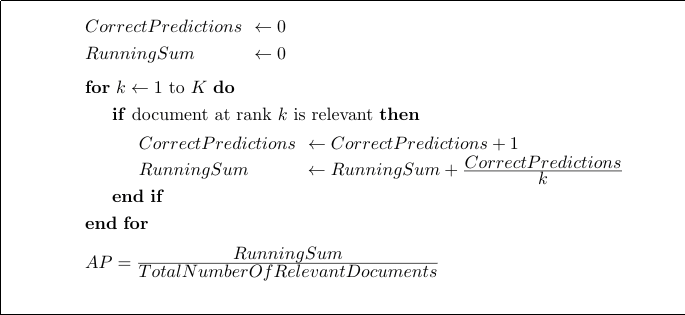 Algorithm for calculating the AP based on a
 ranked list of predictions.
Example: AP Calculated using the algorithm
scores (Sorted)
| k | Document ID |
Predicted Relevance |
Actual Relevance |
|---|---|---|---|
| 1 | 06 | 0.90 | Relevant (1.0) |
| 2 | 03 | 0.85 | Not Relevant (0.0) |
| 3 | 05 | 0.71 | Relevant (1.0) |
| 4 | 00 | 0.63 | Relevant (1.0) |
| 5 | 04 | 0.47 | Not Relevant (0.0) |
| 6 | 02 | 0.36 | Relevant (1.0) |
| 7 | 01 | 0.24 | Not Relevant (0.0) |
| 8 | 07 | 0.16 | Not Relevant (0.0) |
ordered from highest to lowest
Following the algorithm described above, let's go about calculating the AP for our guiding example:
At rank 1:
- \(\text{RunningSum} = 0 + \frac{1}{1} = 1, \text{CorrectPredictions} = 1\)
At rank 2:
- No change. We don't update either the RunningSum or the CorrectPredictions count, since the document at rank 2 is not relevant.
- In other words, we don't count when there's a wrong prediction.
At rank 3:
- \(\text{RunningSum} = 1 + \frac{2}{3} = 1 + 0.666 = 1.666\)
- \(\text{CorrectPredictions} = 2\)
At rank 4:
- \(\text{RunningSum} = 1.666 + \frac{3}{4} = 1.666 + 0.75 = 2.416\)
- \(\text{CorrectPredictions} = 3\)
At rank 5:
- No change, wrong prediction.
At rank 6:
- \(\text{RunningSum} = 2.416 + \frac{4}{6} = 2.416 + 0.66 = 3.076\)
- \(\text{CorrectPredictions} = 4\)
At rank 7:
- No change, wrong prediction.
At rank 8:
- No change, wrong prediction.
And at the end we divide everything by the number of Relevant Documents which is, in this case, equal to the number of correct predictions:
\(AP = \dfrac{\text{RunningSum}}{\text{CorrectPredictions}} \)
\(AP = \dfrac{3.076}{4} \)
\(AP = 0.77\)
DCG: Discounted Cumulative Gain
One advantage of DCG over other metrics is that it also works if document relevances are a real number. In other words, when each document is not simply relevant/non-relevant (as in the example), but has a relevance score instead.
$$ DCG \ @k = \sum\limits_{i=1}^{k} \frac{2^{rel_i} - 1}{log_2(i+1)} $$
where \(rel_i\) is the relevance of the document at index \(i\). Since we're dealing with binary relevances, \(rel_i\) equals 1 if document \(i\) is relevant and 0 otherwise.
scores (Sorted)
| k | Document ID |
Predicted Relevance |
Actual Relevance |
DCG @k |
|---|---|---|---|---|
| 1 | 06 | 0.90 | Relevant (1.0) | 1.0 |
| 2 | 03 | 0.85 | Not Relevant (0.0) | 1.0 |
| 3 | 05 | 0.71 | Relevant (1.0) | 1.5 |
| 4 | 00 | 0.63 | Relevant (1.0) | 1.93 |
| 5 | 04 | 0.47 | Not Relevant (0.0) | 1.93 |
| 6 | 02 | 0.36 | Relevant (1.0) | 2.29 |
| 7 | 01 | 0.24 | Not Relevant (0.0) | 2.29 |
| 8 | 07 | 0.16 | Not Relevant (0.0) | 2.29 |
ordered from highest to lowest
NDCG: Normalized Discounted Cumulative Gain
As you can see in the previous section, DCG either goes up with \(k\) or it stays the same. This means that queries that return larger result sets will probably always have higher DCG scores than queries that return small result sets.
A way to make comparison across queries fairer is to normalize the DCG score by the maximum possible DCG at each threshold \(k\).
$$ NDCG \ @k = \dfrac{DCG \ @k}{IDCG \ @k} $$
Where \(IDCG \ @k\) is the best possible value for \(DCG \ @k\), i.e. the value of DCG for the best possible ranking of relevant documents at threshold \(k\), i.e.:
$$ IDCG \ @k = \sum\limits_{i=1}^{relevant \ documents \\ \, \, \, \, \, \, \, \, \, \, \, \, \, \, \, at \ k} \frac{2^{rel_i} - 1}{log_2(i+1)} $$
scores (Sorted)
| k | Document ID |
Predicted Relevance |
Actual Relevance |
DCG @k | IDCG @k | NDCG @k |
|---|---|---|---|---|---|---|
| 1 | 06 | 0.90 | Relevant (1.0) | 1.0 | 1.0 | 1.0 |
| 2 | 03 | 0.85 | Not Relevant (0.0) | 1.0 | 1.63 | 0.61 |
| 3 | 05 | 0.71 | Relevant (1.0) | 1.5 | 2.13 | 0.70 |
| 4 | 00 | 0.63 | Relevant (1.0) | 1.93 | 2.56 | 0.75 |
| 5 | 04 | 0.47 | Not Relevant (0.0) | 1.93 | 2.56 | 0.75 |
| 6 | 02 | 0.36 | Relevant (1.0) | 2.29 | 2.56 | 0.89 |
| 7 | 01 | 0.24 | Not Relevant (0.0) | 2.29 | 2.56 | 0.89 |
| 8 | 07 | 0.16 | Not Relevant (0.0) | 2.29 | 2.56 | 0.89 |
ordered from highest to lowest
MAP: Mean Average Precision
What about Mean Average Precision (MAP)?
AP (Average Precision) is a metric that tells you how a single sorted prediction compares with the ground truth. E.g. AP would tell you how correct a single ranking of documents is, with respect to a single query.
But what if you need to know how your model's rankings perform when evaluated on a whole validation set? After all, it is really of no use if your trained model correctly ranks classes for some examples but not for others.
This is where MAP (Mean Average Precision) comes in. All you need to do is to sum the AP value for each example in a validation dataset and then divide by the number of examples. In other words, take the mean of the AP over all examples.
So, to summarize:
| AP (Average Precision) | MAP (Mean Average Precision) |
|---|---|
| Informs you how correct a model's ranked predictions are for a single example |
Informs you how correct a model's ranked predictions are, on average, over a whole validation dataset It is a simple average of AP over all examples in a full validation set. |
Average Precision @k
What about AP @k (Average Precision at k)?
Although AP (Average Precision) is not usually presented like this, nothing stops us from calculating AP at each threshold value.
So for all practical purposes, we could calculate \(AP \ @k\) as follows:
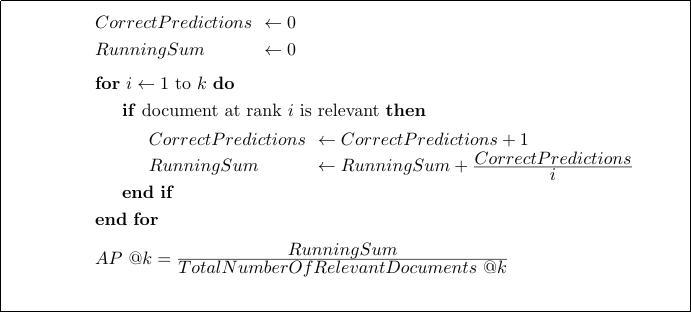 By slightly modifying the algorithm to calculate the
 Average Precision, you can derive AP @k, for varying k
So, using our old guiding example:
scores (Sorted)
| k | Document ID |
Predicted Relevance |
Actual Relevance |
AP @k |
|---|---|---|---|---|
| 1 | 06 | 0.90 | Relevant (1.0) | 1.0 |
| 2 | 03 | 0.85 | Not Relevant (0.0) | 1.0 |
| 3 | 05 | 0.71 | Relevant (1.0) | 0.83 |
| 4 | 00 | 0.63 | Relevant (1.0) | 0.81 |
| 5 | 04 | 0.47 | Not Relevant (0.0) | 0.81 |
| 6 | 02 | 0.36 | Relevant (1.0) | 0.77 |
| 7 | 01 | 0.24 | Not Relevant (0.0) | 0.77 |
| 8 | 07 | 0.16 | Not Relevant (0.0) | 0.77 |
Note that the value at the end is precisely the same as what we got for the full Average Precision
DCG vs NDCG
NDCG is used when you need to compare the ranking for one result set with another ranking, with potentially less elements, different elements, etc.
You can't do that using DCG because query results may vary in size, unfairly penalizing queries that return long result sets.
NDCG normalizes a DCG score, dividing it by the best possible DCG at each threshold.1
| DCG | NDCG (Normalized DCG) |
|---|---|
| Returns absolute values | Returns normalized values |
| Does not allow comparison between queries | Allows comparison between queries |
| Cannot be used to gauge the performance of a ranking model on a whole validation dataset | Can be used to measure a model across a full dataset. Just average NDCG values for each example in the validation set. |
References
Chen et al. 2009: Ranking Measures and Loss Functions in Learning to Rank
- This is interesting because although we use Ranked evaluation metrics, the loss functions we use often do not directly optimize those metrics.
- Published at NIPS 2009
1: Also called the \(IDCG_k\) or the ideal or best possible value for DCG at threshold \(k\).